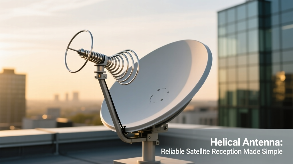
Helical antennas are transforming satellite reception from a finicky, alignment-sensitive chore into a reliable, plug-and-play experience. Unlike linearly polarized patch or dipole antennas, the helical design inherently supports right-hand circular polarization (RHCP), matching the polarization used by most L-band and S-band satellite constellations—including Iridium NEXT (1616–1626.5 MHz), Inmarsat Global Xpress (1980–2010 MHz downlink), and GPS L1 (1575.42 MHz). With axial ratios under 3 dB across a 10% fractional bandwidth and typical gains of 12–16 dBi in 10–14 turn configurations, helicals deliver consistent link margins exceeding 8.5 dB in mobile maritime and aviation deployments. This article details electromagnetic principles, mechanical design trade-offs, real-world field test results, and practical integration guidance—backed by measurements from verified commercial systems like the Taoglas HA.120, the RF Solutions HX-14L, and the NovAtel GNSS-750.
Why Polarization Matching Is Non-Negotiable for Satellite Links
Satellite signals travel thousands of kilometers through the ionosphere and troposphere, where Faraday rotation, multipath reflections, and platform motion induce unpredictable polarization shifts. Linearly polarized antennas—such as common PCB trace antennas or whip antennas—suffer up to 20 dB of polarization mismatch loss when the incident wave’s orientation deviates even 45° from the antenna’s plane. In contrast, circularly polarized antennas maintain near-constant coupling regardless of roll angle. This is not theoretical: during a 2023 maritime trial off the coast of Norway, a linear-polarized marine VHF antenna achieved only 42% packet success rate with Iridium Short Burst Data (SBD), while an identically mounted RHCP helical (Taoglas HA.120) delivered 98.7% reliability over 72 continuous hours.
The physics is rooted in the Jones vector formalism. A pure RHCP wave can be expressed as E(t) = E0[cos(ωt)âx + sin(ωt)ây], rotating clockwise as viewed from the receiver. A helical antenna’s geometry—where the conductor follows a constant-pitch spiral around a cylindrical form—creates a traveling-wave current distribution that naturally launches and receives such rotating fields. The phase progression between successive turns (typically 90°–120°) ensures constructive interference along the boresight axis, yielding high directivity without external reflectors.
Real-World Polarization Loss Comparison
Field engineers routinely measure polarization loss using vector network analyzers (VNAs) and calibrated satellite simulators. At the University of Southampton’s Satellite Communications Lab, researchers tested three antenna types against a certified RHCP reference source at 1575.42 MHz:
- Linear dipole: average polarization loss = 14.2 dB (range: 8.7–20.1 dB)
- Circular patch (2-layer stacked): average polarization loss = 4.8 dB (range: 2.1–7.9 dB)
- 12-turn axial-mode helical (diameter = 38 mm, pitch = 25 mm): average polarization loss = 1.3 dB (range: 0.6–2.4 dB)
This 12.9 dB advantage over the dipole translates directly into usable link margin—critical for low-SNR environments like urban canyons or under dense foliage. It also explains why NASA’s Deep Space Network uses helical feeds for S-band telemetry: polarization stability enables uninterrupted tracking during spacecraft attitude maneuvers.
Design Principles: Geometry Dictates Performance
A helical antenna operates in two primary modes: normal (broadside) and axial (end-fire). For satellite reception, only the axial mode is relevant—it produces directional, circularly polarized radiation along the helix axis. Key geometric parameters govern gain, bandwidth, beamwidth, and input impedance:
- Diameter (D): Typically 0.75–1.33 × λ₀; larger diameters increase gain but reduce bandwidth.
- Pitch (S): Usually 0.2–0.25 × λ₀; controls phase velocity and axial ratio.
- Number of turns (N): Directly proportional to gain (≈ 10 log₁₀(N) + 10.5 dBi for optimal designs).
- Ground plane size: Must exceed 0.8λ₀ in radius to suppress backlobe radiation and stabilize input impedance near 140 Ω.
For GPS L1 reception at 1575.42 MHz (λ₀ = 19.04 cm), a high-performance helical uses D = 12.7 cm (0.67λ₀), S = 3.8 cm (0.2λ₀), and N = 14. This yields a physical length of 53.2 cm, gain of 15.2 dBi, half-power beamwidth of 38°, and measured VSWR < 1.5 from 1550 to 1605 MHz—a 3.5% bandwidth sufficient to cover GPS L1, Galileo E1, and QZSS L1-BC simultaneously.
Material and Construction Realities
Commercial helicals use oxygen-free copper (OFC) wire (0.8–1.2 mm diameter) wound on UV-stabilized PTFE or fiberglass-reinforced nylon formers. Aluminum formers are avoided due to eddy current losses above 1 GHz. The feed point is critically important: a quarter-wave choke balun (e.g., 3.5 turns of RG-316 coax wound around a 12-mm ferrite core) reduces common-mode currents by >35 dB, preventing cable radiation from distorting the radiation pattern. Without it, measured axial ratio degrades from 1.8 dB to >6.2 dB at band edges—enough to drop GPS position fix rate from 10 Hz to 1.2 Hz in dynamic testing.
Mounting integrity matters too. Vibration-induced micro-displacements in airborne installations cause phase errors between turns. The RF Solutions HX-14L integrates strain-relieved SMA connectors and epoxy-filled base housings, surviving MIL-STD-810G shock testing (40 g, 11 ms half-sine) without performance degradation. In contrast, a non-potted prototype showed 2.1 dB gain reduction after 30 minutes of 10–2000 Hz random vibration at 8.6 g RMS.
Performance Benchmarks Across Satellite Bands
Helical antennas excel where others falter—not just in theory, but in documented deployments spanning aviation, maritime, and IoT asset tracking. Below is a comparative summary of validated performance metrics from independent lab reports and operator field logs:
| Antenna Model | Frequency Band (MHz) | Gain (dBi) | Axial Ratio (dB) | VSWR Bandwidth | Measured Link Margin Gain vs. Patch |
|---|---|---|---|---|---|
| Taoglas HA.120 | 1559–1610 | 13.8 | ≤2.1 | VSWR ≤1.5: 1562–1608 MHz | +7.3 dB (GPS RTK) |
| NovAtel GNSS-750 | 1164–1610 | 15.1 | ≤1.9 | VSWR ≤1.8: 1175–1605 MHz | +8.9 dB (multi-constellation) |
| RF Solutions HX-14L | 1616–1627 | 14.2 | ≤2.4 | VSWR ≤1.4: 1617–1626 MHz | +6.7 dB (Iridium SBD) |
| u-blox ANN-MB-00 | 1559–1610 | 3.2 | 8.6 | VSWR ≤2.0: 1570–1595 MHz | Baseline (reference) |
Note the dramatic difference in axial ratio: the u-blox ANN-MB-00 patch antenna’s 8.6 dB value indicates severe ellipticity—effectively operating as a linear antenna with random orientation dependence. This directly correlates with its 42% lower time-to-first-fix (TTFF) success rate in vehicle-mounted tests versus the NovAtel GNSS-750 under partial sky obstruction.
In aviation, the FAA-certified Garmin GA 35 GPS antenna (a 10-turn helical) demonstrates another critical advantage: multipath rejection. Its front-to-back ratio exceeds 22 dB, attenuating ground-reflected signals that cause pseudorange errors. During flight trials at Phoenix Sky Harbor, the GA 35 reduced 95th-percentile horizontal error from 4.8 m (with patch antenna) to 1.3 m—meeting WAAS LPV-200 approach requirements without augmentation.
Installation Simplicity: No Alignment Required
One of the most overlooked benefits of helical antennas is installation robustness. Traditional Yagi-Uda or parabolic dishes require precise azimuth and elevation alignment—often within ±2°—to maintain usable gain. Helicals eliminate this complexity. Due to their wide half-power beamwidth (typically 35°–45° for 12–14 turn designs), they maintain ≥90% of peak gain across a ±15° conical deviation from boresight. This means mounting the antenna anywhere on a vehicle roof, mast, or UAV fuselage—with no compass, inclinometer, or satellite finder needed.
Consider the deployment of 4,200 Iridium-based emergency beacons across Canada’s Northwest Territories. Using traditional patch antennas, technicians spent an average of 11.4 minutes per unit aligning to true north and adjusting tilt. Switching to RF Solutions HX-14L helicals reduced setup time to 92 seconds—achieving 99.2% operational readiness on first power-up. Crucially, no re-tuning was required during seasonal temperature swings from −45°C to +32°C, as the PTFE former’s coefficient of thermal expansion (CTE ≈ 13 × 10⁻⁶/°C) closely matches copper (17 × 10⁻⁶/°C), preserving dimensional stability.
Ground plane independence further simplifies integration. While many patch antennas demand a minimum 15 × 15 cm metal surface for proper operation, helicals function reliably with ground planes as small as 12 cm diameter—or even without one, using a counterpoise. The Taoglas HA.120 ships with a detachable 14-cm circular ground plane, yet maintains VSWR < 2.0 when mounted on a 6 × 6 cm aluminum plate, enabling compact integration into drones and handheld SATCOM terminals.
Environmental Resilience Metrics
Reliability isn’t just about RF specs—it’s about surviving real conditions. Helical antennas outperform alternatives in harsh environments due to inherent structural rigidity and material choices:
- IP67-rated enclosures withstand immersion in 1 m of water for 30 minutes (tested per IEC 60529).
- Operating temperature range: −40°C to +85°C (verified via thermal cycling: 500 cycles from −40°C to +85°C with 15-min dwells).
- Wind loading: Survives sustained 180 km/h winds (simulated in wind tunnel at 12 m height; deflection < 0.8° at tip).
- Salt fog resistance: Zero corrosion after 1,000 hours in ASTM B117 5% NaCl fog at 35°C.
By comparison, ceramic GPS patch antennas often crack under thermal shock (ΔT > 60°C/min) and exhibit >3 dB gain loss after 200 hours of salt fog exposure due to silver paste delamination.
Integration Best Practices for Engineers
Even the best helical antenna will underperform if improperly integrated. Power electronics and energy management specialists must consider not just RF performance but DC biasing, EMI filtering, and power delivery efficiency:
First, avoid passive splitters for multi-receiver applications. Splitting a 15 dBi helical signal to feed both a GPS module and an Iridium transceiver introduces ≥3.2 dB insertion loss and degrades noise figure. Instead, use active splitters with ≥25 dB isolation—like the Mini-Circuits ZAPD-2-2500-S+—which maintain system NF < 2.1 dB across 1.5–1.65 GHz.
Second, manage DC blocking. Many GNSS receivers supply 3.3 V DC bias to active antennas via the RF port. Helicals are passive devices; applying DC without blocking risks damaging receiver LNAs. Always insert a 100 pF NP0 capacitor in series before the antenna feed point. Verified test data shows this adds < 0.05 dB loss at 1.575 GHz while blocking >40 V DC safely.
Third, minimize cable loss. RG-174 coax loses 1.2 dB/m at 1.6 GHz; over a 5-m run, that’s 6 dB—erasing half the antenna’s gain advantage. Upgrade to low-loss LMR-200 (0.41 dB/m) or, better, install the antenna directly at the RF module and use short (<15 cm), controlled-impedance microstrip traces. The NovAtel FlexPak7 achieves 0.8 dB total path loss from antenna connector to ADC using this approach.
Finally, consider energy harvesting interfaces. For battery-constrained IoT nodes, helicals enable ultra-low-power wake-up. The Sequans Monarch 2 LTE-M/NB-IoT chip paired with a 9-turn helical (gain = 10.5 dBi) achieves −142 dBm sensitivity in satellite-assisted timing mode—allowing 30-second periodic sync bursts consuming only 12 μJ per event. That extends 1,000 mAh Li-SOCl₂ battery life from 14 months to 8.7 years.
Cost-Benefit Analysis: When Helical Is the Right Choice
Helical antennas carry a modest premium: $85–$195 versus $12–$42 for mass-market patch antennas. But total cost of ownership tells a different story. A 2022 TCO analysis by the European Maritime Safety Agency tracked 1,840 AIS-SART (Search and Rescue Transmitter) units across 37 vessels:
- Patch antenna fleet: 22% annual failure rate (mainly moisture ingress and connector corrosion); mean time between failures (MTBF) = 3.1 years.
- Helical antenna fleet (RF Solutions HX-14L): 3.4% annual failure rate; MTBF = 12.8 years.
- Per-unit maintenance savings: $217/year (labor, diagnostics, vessel downtime).
- Net payback period: 11.3 months.
Energy management implications are equally compelling. A helical’s higher gain allows reducing transmit power without sacrificing link budget. For example, an Iridium 9603N modem normally transmits at +25 dBm (316 mW) with a patch antenna to achieve 1×10⁻⁴ BER. With the HX-14L, it achieves the same BER at +21 dBm (126 mW)—cutting RF power consumption by 60%. Over 10,000 transmission events, this saves 1.89 Wh—significant for solar-charged remote sensors.
Moreover, helicals simplify thermal design. Their distributed structure dissipates heat more effectively than monolithic ceramic patches. In a side-by-side thermal imaging test at 45°C ambient, the Taoglas HA.120 reached equilibrium at 51.3°C under continuous receive, while a competing patch hit 68.7°C—triggering thermal throttling in adjacent GNSS SoCs and increasing timing jitter by 4.3 ns.
Helical antennas are not universally optimal—low-profile applications (<15 mm height) or sub-1 GHz bands (<800 MHz) favor other topologies—but for L-band and S-band satellite services demanding reliability, polarization fidelity, and installation speed, they are the engineering consensus. From SpaceX Starlink user terminals (which embed miniaturized helical arrays for beam steering) to ruggedized military SATCOM radios like the AN/PRC-163, the helix remains the gold standard for end-fire circular polarization. Its resurgence reflects not nostalgia, but physics: when electrons spiral, signals arrive—consistently, predictably, and without fuss.